JHU-Table-Setting Dataset:

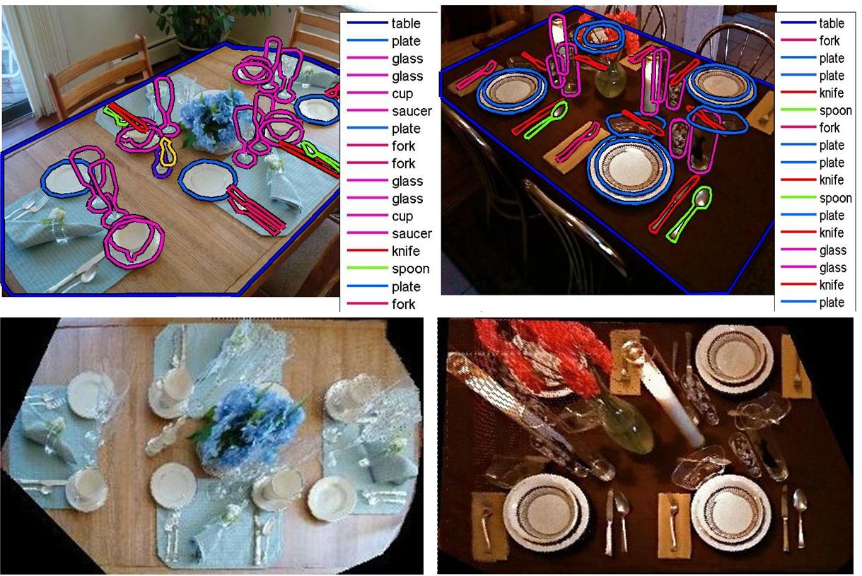
We collected and annotated about 3000 images of table setting scenes with more than 30 object categories. The images in this dataset were collected from multiple sources such as Google, Flickr, Altavista, etc. The annotation task was carried out by three annotators over a period of about ten months using the LabelMe online annotating website. The consistency of labeled images were then verified and synonymous labels were consolidated. The annotation of this dataset was done with careful supervision resulting in high quality annotations, better than what we normally get from Amazon Mechanical Turk. Figure below shows a snapshot of the ‘‘JHU Table-Setting Dataset’’:

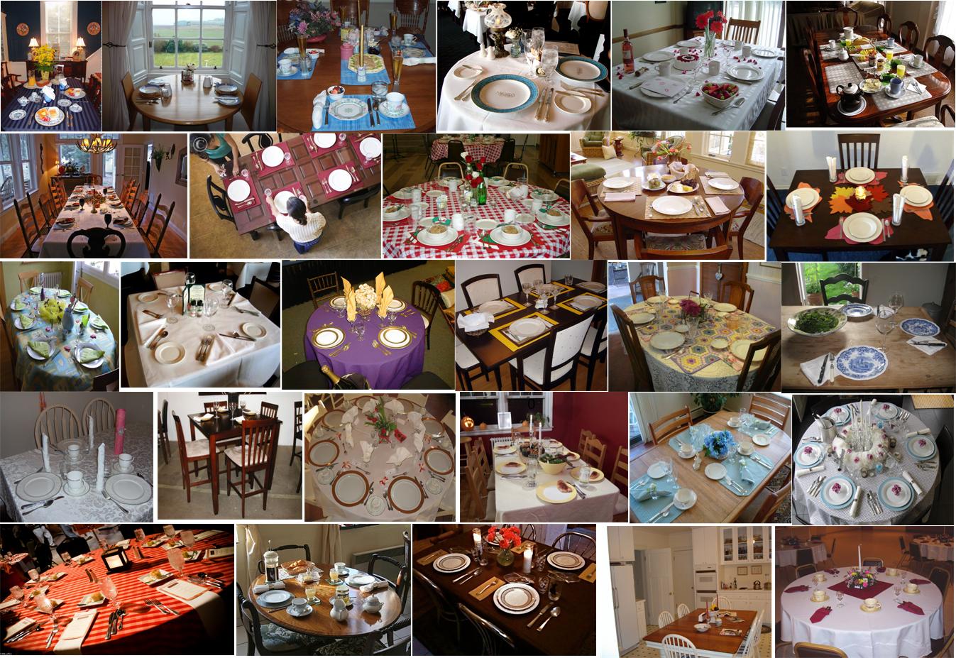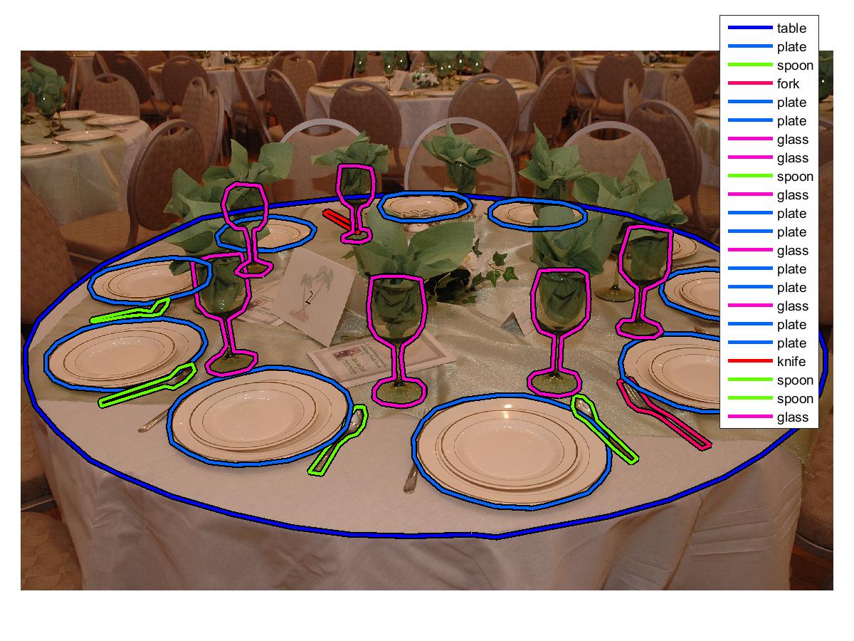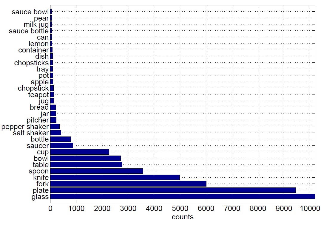
Figure below shows the number of annotated instances per object category in the whole dataset for the 30 top most annotated object categories:

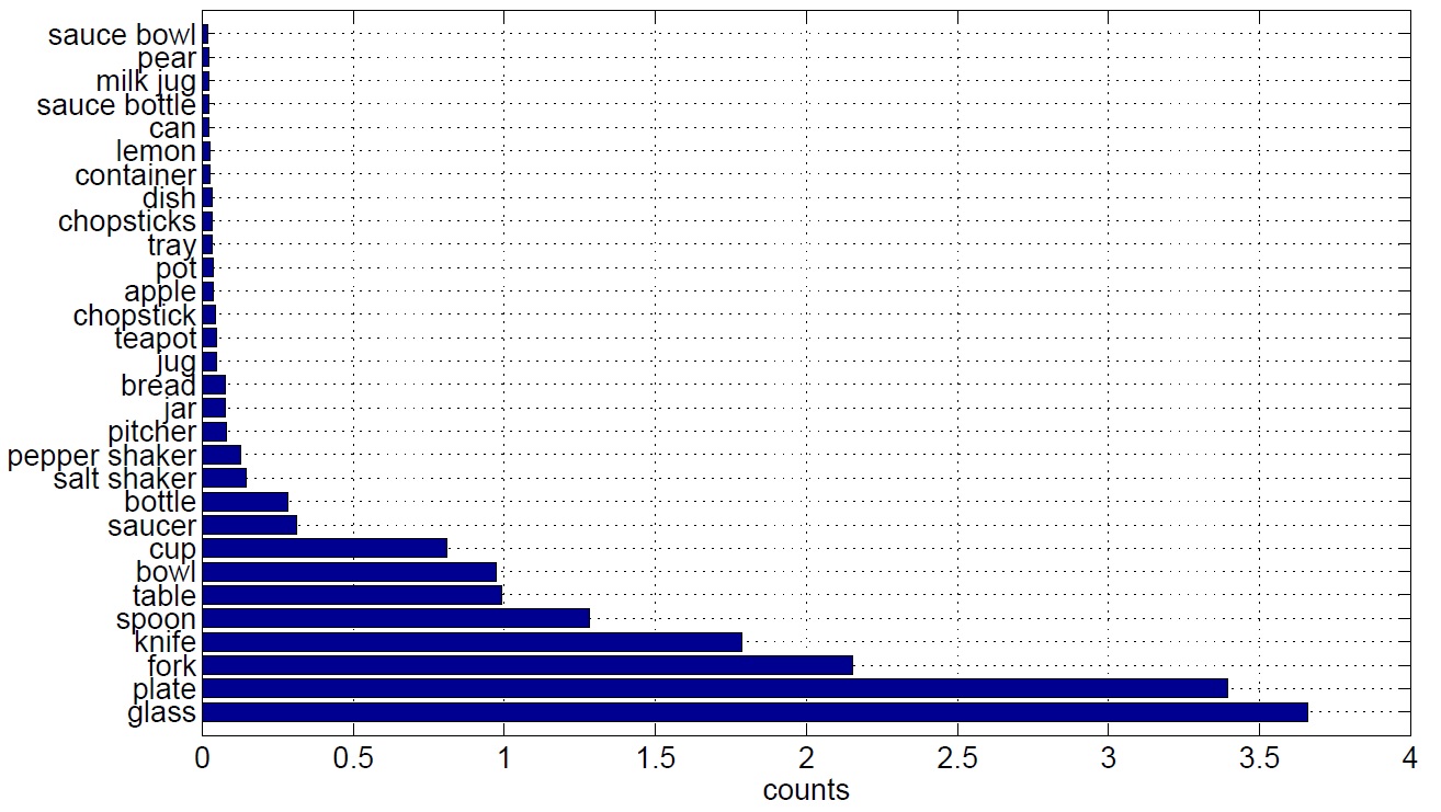
The average number of annotations per image is about 17. The average number of annotated instances per object category per image is shown in below:

Additionally, the Homography matrix for every image in the dataset is manually estimated. To estimate the homography (up to scale) at least four pairs of corresponding points are needed according to the Direct Linear Transformation (DLT) algorithm (see page 88 of book by Hartley and Zisserman). These four pairs of corresponding points were located in the image coordinate system by annotators’ best visual judgment about four corners of a square in real world whose center coincides with the origin of the table (world) coordinate system. We are able to undo the projective distortion due to the perspective effect by back-projecting the table surface in the image coordinate system onto the world coordinate system. The homography matrices are scaled appropriately (using object's typical sizes in real world) such that after back-projection the distance of object instances in the world coordinate system (measured in meters) can be computed. Figure below shows two typical images from this dataset and their rectified versions:

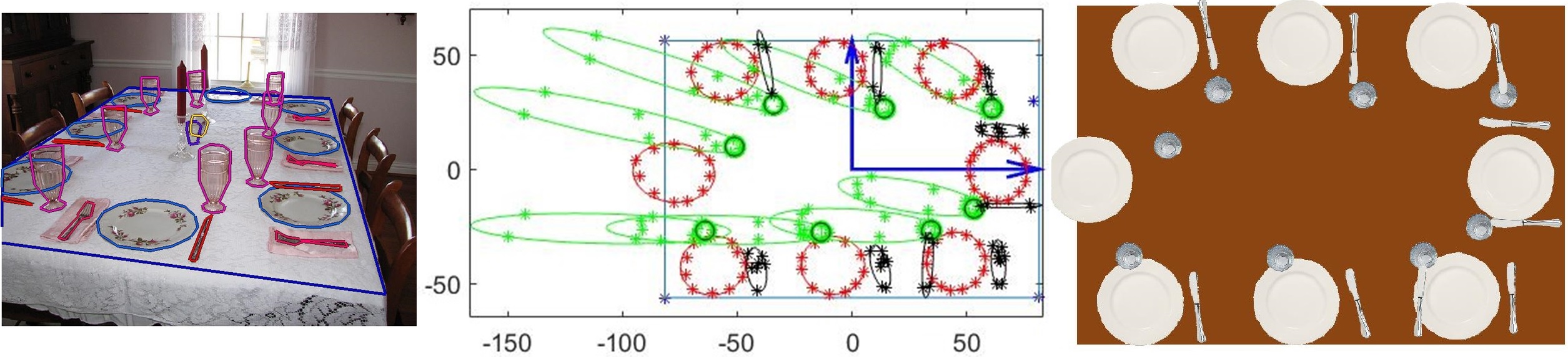
Each object instance was annotated with an object category label plus an enclosing polygon. An ellipse can be fit to the vertices of the polygon to estimate the object's shape and pose in the image plane. Figure below (left) shows an example annotated image; Figure below (middle) shows the corresponding back-projection of vertices of annotation polygons for plates (in textcolor{red}{red}

), glasses (in textcolor{green}{green}

), and utensils (in textcolor{black}{black}

). Note that non-planar objects (e.g. glass) often get distorted after back projection (e.g. elongated green ellipses) since the homography transformation is a perspective projection from points on the table surface to the camera's image plane. Hence, we estimated the base of vertical objects (shown by black circles in the middle figure) to estimate their location in the table (world) coordinate system since the center of fitting ellipse to the back-projection of such objects’ annotation points is not a good estimate of their 3D location in the real world. Figure below (right) shows top-view visualization of the annotated scene in the left using top-view icons of the corresponding object instances for plates, glasses, and utensils (note that all utensil instances are shown by top-view knife icons).

Download:

clear
clc

addpath('D:\LabelMeToolbox-master\install');
addpath('D:\LabelMeToolbox-master\main');
addpath('D:\LabelMeToolbox-master\XMLtools')
addpath('D:\LabelMeToolbox-master\querytools');

folderlist = {'sandbox/mt_static_submitted_Ehsan_Jahangiri_kitchen_setting_google_search_aug_2011',...
    'sandbox/mt_static_submitted_Ehsan_Jahangiri_kitchen_setting_oct_2011',...
    'sandbox/mt_static_submitted_Ehsan_Jahangiri_table_setting_dec_2011',...
    'sandbox/mt_static_submitted_Ehsan_Jahangiri_table_setting_set_2_dec_2011',...
    'sandbox/mt_static_submitted_Ehsan_Jahangiri_table_setting_set_3_dec_2011',...
    'sandbox/mt_static_submitted_Ehsan_Jahangiri_table_setting_set_4_jan_2012',...
    'sandbox/mt_static_submitted_Ehsan_Jahangiri_table_setting_set_5_feb_2012',...
    'sandbox/mt_static_submitted_Ehsan_Jahangiri_table_setting_set_6_feb_2012',...
    'sandbox/mt_static_submitted_Ehsan_Jahangiri_table_setting_set_7_march_2012',...
    'users/JHUEhsan//sandboxmt_static_submitted_hsan_ahangiri_table_setting_set_8_jun_2012',...
    'users/JHUEhsan//sandboxmt_static_submitted_ehsan_jahangiri_table_setting_set_9_ug_2012'};

HOMEIMAGES = 'D:\Labelme_download_table\images';
HOMEANNOTATIONS = 'D:\Labelme_download_table\annotations';

% Download the whole images
LMinstall(folderlist, HOMEIMAGES, HOMEANNOTATIONS);

%==================================
% After putting all images and xml files in one single folder run the following script:
% HOMEIMAGES = 'D:\DataSet\All_Images';
% HOMEANNOTATIONS = 'D:\DataSet\All_Annotations';
% D = LMdatabase(HOMEANNOTATIONS, HOMEIMAGES);
% save('AnnotTableSetNov2015.mat','D')

Example Matlab script for reading an image annotation and measuring its table area in $cm^{2}$ :

% ===== some commands ==========
% D(imgnum).annotation.folder
% D(imgnum).annotation.filename
% D(imgnum).annotation.object(objectnum).name
% D(imgnum).annotation.object(objectnum).polygon
% ===================================

clc
clear

addpath('D:\LabelMeToolbox') 	     			% adding path to the functions we use from the toolbox
load('AnnotTableSetNov2015.mat','D')   			% load annotations
load('Homography_All_in_One.mat','HH','What_img')	% load homographies

starting_img = 5201;					% the first image's index
ending_img = 8317;					% the last image's index
size_mismatch_ratio = 2.5;				% scale mismatch (always include)
n = 1;				     			% image index

D(n).annotation.filename				% print filename
[Dn, jn] = LMquery(D(n), 'object.name', 'table');       % query "table category"

if (~isempty(jn) && str2num(Dn.annotation.filename(1:4)) == (starting_img+n-1) ),  % check if the image has been annotated and the index is correct.

    H2cm = inv(HH(:,:,n));     				% invert the homography matrix for back-projection (pixel to centimeters)

    X = Dn(1).annotation.object(1).polygon.y;		% inversion of x-y coordinates for compatibility
    Y = Dn(1).annotation.object(1).polygon.x;
    ObjOutline = [X';Y';ones(1,length(X))];		% homogeneous coordinates
    TrnsObjOutline = H2cm*ObjOutline./(repmat([0,0,1]*H2cm*ObjOutline,3,1));  % back-projection.

    XTr = size_mismatch_ratio*TrnsObjOutline(1,:)';	% correcting scale mismatch
    YTr = size_mismatch_ratio*TrnsObjOutline(2,:)';	% correcting scale mismatch

    Image(n).TrueArea = polyarea(XTr,YTr);		% measuring the area of table in cm^2.

end

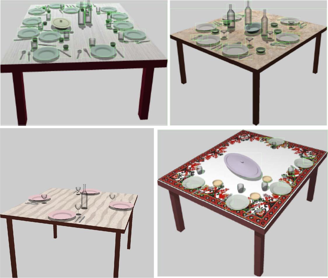
Synthetic Table-Setting Scene Renderer:

This synthetic image renderer (developed by Erdem Yoruk) inputs the camera's calibration parameters, six rotation and translation camera's extrinsic parameters, table length and width, and 3D object poses in the table's coordinate system and outputs the corresponding table setting scene. Figure below shows some synthetic images generated by this renderer.

Download:

Citation:

This dataset is for non-commercial research use. Please cite the following papers if you used the “JHU-Table-Setting” dataset in your publication:

Questions:

For questions please contact me by email (ejahang1 [@] jhu [DOT] edu) and I will try to respond as quick as possible.