Notes
The Palest Ink is Better than the Best Memory!
As the Chinese proverb goes, the palest ink is better than the best memory. It is always better to put things that you want to remember down in writing than to refer to a memory. Years ago, I used Google Notebook to jot down things I find useful on the Internet. After Google announced that they were planning to shut down the service, I switched to Evernote. Evernote is in fact much better than Google Notebook. Besides the basic functionalities that Google Notebook has, Evernote provides many other useful features. For example, you can use your Smartphone to take a picture of your meeting notes on the whiteboard, and the (picture) note will be synced seamlessly across all the devices on which you have an working Evernote client, as well as the Evernote server. The coolest part is that all your notes, including your hand-written picture notes, your pdf notes, are searchable. Despite of all its useful and cool features, there is one thing that I need badly but Evernote doesn't have---LaTeX support. Since I'm a Statistician, from time to time, I want to jot down a note with mathematical formulas, but it is unwieldy to do in Evernote. Emacs orgmode is another tool I've been using for organizing notes, todos, and other plain text documents. It is really powerful---as the website mentions, the typical answer to "Can it (orgmode) do X?" is "Yes!". This website is published through Emacs orgmode.Bias–Variance Analysis in Regression
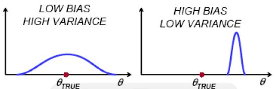
Suppose the ture function is \(Y = f(X) + \epsilon\), where \(\epsilon \sim N(0, \sigma^2)\). Given a set of training example, \(T = \{(x_i, y_i)\}\), we fit a hyphothesis \(\hat{f}\) to the data to minimize the squared error \(\sum_i (y_i-\hat{f}(x_i))^2\). For a fixed point \(x_0\), \(\hat{f}(x_0)\) is a random variable, where the randomness comes from the randomness in the traning set. The expected prediction error (EPE) at a fixed point \(x_0\) can be decomposed as:
\[ \begin{aligned} EPE(x_0) & = E_{Y, T} \left[\left(Y - \hat{f}(x_0)\right)^2\right] \\ & = E_{Y, T} \left[\left( (Y - f(x_0)) - (\hat{f}(x_0) - E_T[\hat{f}(x_0)]) - (E_T[\hat{f}(x_0)] - f(x_0)) \right)^2\right] \\ & = E_{Y} \left[\left(Y - f(x_0)\right)^2\right] + E_{T} \left[\left(\hat{f}(x_0) - E_T[\hat{f}(x_0)]\right)^2\right] + \left(E_T[\hat{f}(x_0)] - f(x_0)\right)^2 \\ & = \sigma^2 + Var_{T}\left(\hat{f}(x_0)\right) + \left(bias(\hat{f}(x_0))\right)^2 \end{aligned} \] There are three terms in the EPE decomposition. The first term \(\sigma^2\) is the output variance (\(f(x_0) = E[Y]\)), and is beyond our control. It is called the irreducible error. The second and third terms are under our control, and make up the mean squared error of \(\hat{f}(x_0)\) in estimating \(f(x_0)\):
\[ MSE\left(\hat{f}(x_0)\right) = E_T\left[\left(\hat{f}(x_0) - f(x_0)\right)^2\right]. \] The second term is the variance component of MSE, and is determined by how the prediction varies around its average prediction. The bias component of MSE is the squared difference between the true mean \(f(x_0)\) and the expected value of the estimate, where the expectation averages the randomness in the training data.
As model complexity increases, \(\hat{f}\) fits a given training sample better and better. Consequently, the preditions (of a same point) resulting from different training samples differ more from each other. That is, the variance compoent increases as the model complexity increases. On the other hand, the expected prediction tends to be close to the true mean \(f(x_0)\) as we fit training samples better and better. Imagine that \(\hat{f}\) fit all training samples perfectly, then the bias would be zero.
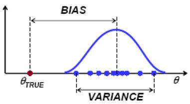
Bias: How close is the average estimate to the true value. $$Bias(\hat{\theta}) = E[\hat{\theta}] - \theta.$$ Variance: How much does the estimate change for different training samples
Install R Package Rmpi in Ubuntu
I tried to install the R package Rmpi and got the following error
...
configure: error: "Cannot find mpi.h header file"
ERROR: configuration failed for package 'Rmpi'
* removing '/usr/local/lib/R/site-library/Rmpi'
...
After researching online, I found I need to install some dependencies
sudo apt-get build-dep r-cran-rmpi
ANOVA Unbalance Data: Types of Sums of Squares (reference)
By converting categorical variables into dummy indicator variables, an ANOVA can be written as a general linear model $$Y = X\beta + \varepsilon.$$ The design matrix \(X\) for a 2-way ANOVA with factorial design 2x3 looks like
Data                      Design Matrix
             A        B                      A*B
A B     mu A1 A2   B1 B2 B3   A1B1 A1B2 A1B3 A2B1 A2B2 A2B3
1 1      1  1  0    1  0  0      1    0    0    0    0    0
1 2      1  1  0    0  1  0      0    1    0    0    0    0
1 3      1  1  0    0  0  1      0    0    1    0    0    0
2 1      1  0  1    1  0  0      0    0    0    1    0    0
2 2      1  0  1    0  1  0      0    0    0    0    1    0
2 3      1  0  1    0  0  1      0    0    0    0    0    1
After removing an effect of a factor or an interaction from the above full model (i.e. deleting some columns from the matrix X), we obtain an increased error due to the removal of the effect.
Splitting a Vector (reference)
Problem: Split a vector whenever an element in the vector is smaller than its predecessor.
f <- function(x) {
  ix <- cumsum(diff(c(x[1], x)) < 0)
  split(x, ix)
}

> x <- c(1,1,2,3,4,5,1,2,3,2,3,4,5,6,4,5)
> f(x)
$`1`
[1] 1

$`2`
[1] 1 2 3 4 5

$`3`
[1] 1 2 3

$`4`
[1] 2 3 4 5 6

$`5`
[1] 4 5
Oracle With Clause, Inline View and Subquery
With Clause
WITH t1 AS
(SELECT select_list
   FROM ...)
, t2 AS
(SELECT select_list
  FROM ...)
SELECT select_list
  FROM t1, t2
...
Inline View
An inline view is a SELECT statement in the FROM clause of another SELECT statement. For example, the following query finds the employees who earn the highest salary in each department.
SELECT a.last_name, a.salary, a.department_id, b.maxsal
  FROM employees a,
       (SELECT department_id, max(salary) maxsal
          FROM employees
         GROUP BY department_id) b
 WHERE a.department_id = b.department_id
   AND a.salary = b.maxsal;
We can use the with clause to achieve the same goal.
WITH b AS
(SELECT department_id, max(salary) maxsal
   FROM employees
  GROUP BY department_id)
SELECT a.last_name, a.salary, a.department_id, b.maxsal
  FROM employees a, b
 WHERE a.department_id = b.department_id
   AND a.salary = b.maxsal;
Subquery
A subquery is a SELECT statement in the WHERE or HAVING clause of another SELECT statement. A subquery processes as follows:
- Simple Subquery: the inner query (i.e. subquery) is processed first, the results are returned to the outer query and then the outer query is processed.
- Correlated Subquery: outer -> inner -> outer -> inter -> outer …
SELECT last_name, salary, department_id
  FROM employees a
 WHERE salary = (SELECT max(salary)
                   FROM employees b
                  WHERE b.department_id = a.department_id);
SQL Joins (reference)
A JOIN is a query that combines rows from two or more tables or views. Oracle Database performs a join whenever multiple tables appear in the FROM clause. Most join queries contain at least one join condition, which compares two columns, each from a different table. To execute a join, Oracle Database combines pairs of rows, each containing one row from each table, for which the join condition evaluates to TRUE.
To execute a join of three or more tables, Oracle first joins two of the tables based on the join conditions comparing their columns and then joins the result to another table based on join conditions containing columns of the joined table and the new table. This process is repeated until all tables are joined into the result. The optimizer determines the order in which Oracle joins tables based on the join condition, indexes on the tables, and, any available statistics for the tables.
The result of a join can be defined as the outcome of first taking the Cartesian product of all records in the tables, then returning all records that satisfy the join condition.
- Inner Join is a join of two or more tables that returns only those rows that satisfy the join conditions.
- Outer Join extends the result of an inner join by returning all rows that satisfy the join condition, as well as some or all of those rows from one table for which no rows from the other table satisfy the join condition.
- To write a query that performs an outer join of tables A and B and returns all rows from A, use the LEFT OUTER JOIN syntax in the FROM clause, or apply the outer join operator (+) to all columns of B in the join condition in the WHERE clause.
The outer join operator (+) should be placed on the side of the operator (e.g. "=") where we want to have nulls returned if no value matches. However Oracle recommends to use the FROM clause OUTER JOIN syntax rather than the Oracle join operator.
Dates and Times in R (reference)
Dates to and from Characters
- as.Date converts character strings to Date objects, which are stored
internally as the number of days or seconds from some reference date.
# Usage: as.Date(x, format=...)
x <- as.Date("2012-01-01", format="%Y-%m-%d") as.integer(x) [1] 15340
as.Date("2012-01-01", format="%Y-%m-%d") - 15340 [1] "1970-01-01"
If the input dates are not in the standard format, a format string can be composed using the following elements
%a Abbreviated weekday name A Full weekday name b Abbreviated month name
%B Full month name d Day of the month as decimal number (01-31)
%j Day of year as decimal number (001-366)
%m Month as decimal number (01-12)
%x Date.  Locale-specific on output, '"%y/%m/%d"' on input
%y Year without century (00-99). Values 00 to 68 are prefixed by 20 and 69 to 99 by 19
%Y Year with century
as.Date accepts numeric input (the number of days since an epoch) if 'origin' is supplied
as.Date(10, origin="2000-01-01") [1] "2000-01-11"
- format and as.character convert a Date object to a character string
as.character(as.Date("2012-01-01", format="%Y-%m-%d"), format="%A") [1] "Sunday" format(as.Date("2012-01-01", format="%Y-%m-%d"), format="%B %d, %A") [1] "January 01, Sunday" - Date-Time classes, POSIXlt and POSIXct, handle calendar dates and times
(to the nearest second). POSIX represents a Portable Operating System
Interface, primarily for UNIX systems, but available on other operating
systems as well. The two POSIX date/time classes differ in the way that
the values are stored internally. The POSIXct class stores date/time
values as the number of seconds since January 1, 1970, while the POSIXlt
class stores them as a list with elements for second, minute, hour, day,
month, and year, among others. Unless you need the list nature of the
POSIXlt class, the POSIXct class is the usual choice for storing dates in
R. Examples of valid POSIX date or date/time inputs include:
# 1915/6/16
# 2005-06-24 11:25
# 1990/2/17 12:20:05
# 2005-10-28 07:30:05 PDT
Functions for POSIX classes include: as.POSIXct, as.POSIXlt, structure, etc.
dts <- c("2005-10-21 18:47:22","2005-12-24 16:39:58", "2005-10-28 07:30:05 PDT")
as.POSIXct(dts)
mydates <- dts
class(mydates) <- c("POSIXct", "POSIXlt")
Assigning a Vector to Every Element of a List
- Method 1
> a <- vector("list", 3) > a[] <- list(1:3) > a [[1]] [1] 1 2 3 [[2]] [1] 1 2 3 [[3]] [1] 1 2 3 - Method 2
a <- lapply(1:3, function(x) 1:3)
> a
[[1]]
[1] 1 2 3

[[2]]
[1] 1 2 3

[[3]]
[1] 1 2 3
Send Output to a Character String or File
capture.output converts the output that you want to print to file to a text string. Then you can simply cat the output to the file.
# Usage
# capture.output(..., file = NULL, append = FALSE)

> x <- capture.output(1:5)
> x
[1] "[1] 1 2 3 4 5"
Decision Tree/Random Forest Split-Stopping Criteria
Gini impurity
The Gini coefficient (or index) measures the inequality among values of a frequency distribution (for example levels of income). A Gini coefficient of zero expresses perfect equality where all values are the same. A Gini coefficient of one expresses maximal inequality among values (for example only one person has all the income).
Gini impurity for a node t is defined as
$$Gini(t) = 1 - \sum_j [prob(j | t)]^2$$
where p(j|t) si the relative frequency of class j at node t.
- maximum = 1 - 1/n when all instances are equally distributed among all classes, implying least interesting information
- minimum = 0 when all instances belong to one class, implying most interesting information
When a node t is split into k children nodes, the quality of the split is computed as
$$Gini(split) = \sum_{i=1}^k Gini(i) \frac{n_i} {n}$$
where \(n_i\) is the number of instances in child i.
Entropy
The entropy at a given node t is
$$Entropy(t) = - \sum_j p(j | t) \log p(j|t)$$
Entropy measures homogeneity of a node.
- maximum = \(\log n_c\), when instances are equality distributed among all classes, implying least information
- minimum = 0, when all instances belong to one class, implying most information
When a node t is split into k children nodes, the quality of the split is computed as
$$Entropy(split) = \sum_{i=1}^k Entropy(i) \frac{n_i} {n}$$
Information Gain
The information gain measures the reduction in Entropy from splitting a parent node t into k children nodes. It is defined as:
$$Gain(split) = Entropy(t) - \left(\sum_{i=1}^k Entropy(i) \frac{n_{i}} {n}\right)$$
Classification Error
$$Error(t) = 1 - \max_i p(i | t)$$
- maximum = \(1 - 1/n_c\), when all instances are equally distributed among all classes, implying least information
- minimum = 0, when all instances belong to one class, implying most information
Deviance
$$D(y) = - 2\left(log(p(y | \hat{\theta}_0)) - log(p(y | \hat{\theta}_s))\right)$$
Bootstrapping, Boosting and Bagging
Bootstrapping
The phrase "pull yourself up by your bootstraps" refers to boots and their straps (laces) and to the imagined feat of a lifting oneself off the ground by pulling on one's bootstraps. This impossible task is supposed to exemplify the achievement in getting out of a difficult situation by one's own efforts. In statistics, bootstrapping is a method for assigning measures of accuracy to sample estimates. This technique allows estimation of the sampling distribution of almost any statistic using only very simple methods. Generally, it falls in the broader class of resampling methods.
Assume we are interested in the average height of people worldwide. We cannot measure all the people in the global population, so instead we sample only a tiny part of it, and measure that. Assume the sample is of size N; that is, we measure the heights of N individuals. From that single sample, only one value of the mean can be obtained. In order to reason about the population, we need some sense of the variability of the mean that we have computed. To use the simplest bootstrap technique, we take our original data set of N heights, and, using a computer, make a new sample (called a bootstrap sample) that is also of size N. This new sample is taken from the original using sampling with replacement so it is not identical with the original "real" sample. We repeat this a lot (maybe 1000 or 10,000 times), and for each of these bootstrap samples we compute its mean (each of these are called bootstrap estimates). We now have a histogram of bootstrap means. This provides an estimate of the shape of the distribution of the mean from which we can answer questions about how much the mean varies. (The method here, described for the mean, can be applied to almost any other statistic or estimator.)
*The key principle of the bootstrap is to provide a way to simulate repeated observations from an unknown population using the obtained sample as a basis.*
Case Resampling The Monte Carlo algorithm for case resampling is quite simple. First, we resample the data with replacement, and the size of the resample must be equal to the size of the original data set. Then the statistic of interest is computed from the resample from the first step. We repeat this routine many times to get a more precise estimate of the Bootstrap distribution of the statistic. The 'exact' version for case resampling is similar, but we exhaustively enumerate every possible resample of the data set.
Smooth Bootstrap Under this scheme, a small amount of (usually normally distributed) zero-centered random noise is added on to each resampled observation. This is equivalent to sampling from a kernel density estimate of the data.
Parametric Bootstrap In this case a parametric model is fitted to the data, often by maximum likelihood, and samples of random numbers are drawn from this fitted model. Usually the sample drawn has the same sample size as the original data. Then the quantity, or estimate, of interest is calculated from these data. This sampling process is repeated many times as for other bootstrap methods. The use of a parametric model at the sampling stage of the bootstrap methodology leads to procedures which are different from those obtained by applying basic statistical theory to inference for the same model.
Boosting
Boosting is a machine learning meta-algorithm for performing supervised learning. Boosting is based on the question posed by Michael Kearns: Can a set of weak learners create a single strong learner? A weak learner is defined to be a classifier which is only slightly correlated with the true classification (it can label examples better than random guessing). In contrast, a strong learner is a classifier that is arbitrarily well-correlated with the true classification.
While boosting is not algorithmically constrained, most boosting algorithms consist of iteratively learning weak classifiers with respect to a distribution and adding them to a final strong classifier. When they are added, they are typically weighted in some way that is usually related to the weak learners' accuracy. After a weak learner is added, the data is reweighted: examples that are misclassified gain weight and examples that are classified correctly lose weight (some boosting algorithms actually decrease the weight of repeatedly misclassified examples, e.g., boost by majority and BrownBoost). Thus, future weak learners focus more on the examples that previous weak learners misclassified.
The main variation between many boosting algorithms is their method of weighting training data points and hypotheses. AdaBoost is very popular and perhaps the most significant historically as it was the first algorithm that could adapt to the weak learners. However, there are many more recent algorithms such as LPBoost, TotalBoost, BrownBoost, MadaBoost, LogitBoost, and others.
Bagging
Bootstrap aggregating (bagging) is a machine learning ensemble meta-algorithm to improve machine learning of statistical classification and regression models in terms of stability and classification accuracy. It also reduces variance and helps to avoid overfitting. Given a standard training set D of size n, bagging generates m new training sets Di, each of size n' > n, by sampling examples from D uniformly and with replacement. By sampling with replacement, it is likely that some examples will be repeated in each Di. If n'=n, then for large n the set Di is expected to have 63.2% of the unique examples of D, the rest being duplicates. This kind of sample is known as a bootstrap sample. The m models are fitted using the above m bootstrap samples and combined by averaging the output (for regression) or voting (for classification).
Since the method averages several predictors, it is not useful for improving linear models. Similarly, bagging does not improve very stable models like k nearest neighbors.
Quantiles
Quantiles are points taken at regular intervals from the cumulative distribution function (CDF) of a random variable. Dividing ordered data into q essentially equal-sized data subsets is the motivation for q-quantiles; the quantiles are the data values marking the boundaries between consecutive subsets. Put another way, the kth q-quantile for a random variable is the value x such that the probability that the random variable will be less than x is at most k/q and the probability that the random variable will be more than x is at most (q-k)/q. There are q-1 of the q-quantiles, one for each integer k satisfying 0 < k < q.
"rm -rf filename" complains "permission denied"
"rm -rf filename" complains "permission denied" even I have write permission to the file. In UNIX and Linux, the ability to remove a file is not determined by the access bits of that file. It is determined by the access bits of the directory which contains the file. Think of it this way – deleting a file doesn't modify that file. You aren't writing to the file, so why should "w" on the file matter? Deleting a file requires editing the directory that points to the file, so you need "w" on the that directory.
Compile Unison Under Cygwin
- Install Cygwin packages: make, ocaml and ctags
- Download Unison here
- make UISTYLE=text
Remark: You might meet the following error
Makefile.OCaml:343: recipe for target `update.cmx' failed
make: *** [update.cmx] Error 2
If that is the case, change the 4th line of update.mli from
module NameMap : Map.S with type key = Name.t
to
module NameMap : MyMap.S with type key = Name.t
Cygwin "Could not create directory 'xxx/xxx.ssh'" Error
Every now and then, ssh gives me the error "Could not create directory 'xxx/xxx.ssh'". OpenSSH under Cygwin uses the /etc/passwd file to determine your HOME directory, NOT whatever you might have set for HOME as an environment variable, either inside of your BASH shell or in Windows itself. The answer is to patch the /etc/passwd file to have a correct directory. I.e., open /etc/passwd and replace the text /home/YOUR_NAME with your $HOME directory.
Setting Paths for R and Aspell in Cygwin
(if (string-equal system-type "cygwin")
  (progn
    (setq-default inferior-R-program-name "/cygdrive/c/Program Files/R/R-2.14.0/bin/x64/Rterm.exe")
    (setq ispell-program-name "/cygdrive/c/Program Files/Aspell/bin/Aspell.exe"))
nil)

(if (string-equal system-type "windows-nt")
  (progn
    (setq-default inferior-R-program-name "C:\\Program Files\\R\\R-2.14.0\\bin\\x64\\Rterm.exe")
    (setq ispell-program-name "C:\\Program Files\\Aspell\\bin\\Aspell.exe"))
nil)
Remapping Keys Using AutoHotkey
AutoHotkey is a must-have tool to me. Here are some of the tricks I use:
;; Change Capslock to control and change right control to capslock
Capslock::Ctrl
RCtrl::Capslock
;; Change control-space to control-@
^Space::^@
;; Change shift-space to shift-left_alt. Control Panel -> Change keyboard or
;; other input methods -> Change Keyboards -> Advanced Key Settings: change the
;; key sequence for "between input languages" to "Left Alt + Shift"
+Space::+LAlt
Orgmode math formatting in HTML export
- Download the current version of MathJax at here.
- Extract the downloaded file to the public_html folder.
- Add the following to header of your org file
#+MATHJAX: align:"center" mathml:t path:"mathjax-MathJax-07669ac/MathJax.js"
# Other options could be align:"left" indent:"5%"
Easy Templates in Emacs org-mode
To insert a template (e.g. #+BEGIN_SRC and #+END_SRC pairs) in org-mode, type a "<", followed by a template selector and <TAB>. Completion takes effect only when the keystrokes (e.g. "<s") are typed on a line by itself. The following template selectors are currently supported:
s     #+begin_src     ... #+end_src
e     #+begin_example ... #+end_example
q     #+begin_quote   ... #+end_quote
v     #+begin_verse   ... #+end_verse
c     #+begin_center  ... #+end_center
l     #+begin_latex   ... #+end_latex
L     #+latex:
h     #+begin_html    ... #+end_html
H     #+html:
a     #+begin_ascii   ... #+end_ascii
A     #+ascii:
i     #+index: line
I     #+include: line
LaTeX Specific Header in an Org File
#+OPTIONS: LaTeX:t          Do the right thing automatically (MathJax)
#+OPTIONS: LaTeX:dvipng     Force using dvipng images
#+OPTIONS: LaTeX:nil        Do not process LaTeX fragments at all
#+OPTIONS: LaTeX:verbatim   Verbatim export, for jsMath or so
Insert the Current Date When Publishing an org File
#+:DATE %b %d, %Y
%a    the abbreviated name of the day of week
%A    the full name of the day of week
%b    the abbreviated name of the month
%B    the full name of the month
%d    the day of month, zero-padded
%H    the hour (00-23)
%I    the hour (01-12)
%j    the day of the year (001-366)
%k    the hour (0-23), blank padded
%l    the hour (1-12), blank padded
%m    the month (01-12)
%M    the minute (00-59)
%n    a newline
%p    "AM" or "PM", as appropriate
%S    the seconds (00-59)
%t    a tab character
%W    the week of the year (01-52), assuming that weeks start on Monday
%y    the year without century (00-99)
%Y    the year with century
%Z    the time zone abbreviation (e.g., "EST")
%z    the time zone numerical offset (e.g., "-0500")