The Swiss Roll Matching Example

Load the Swiss Roll data from the 3D nonlinear Swiss Roll and its 2D linear generating data, do manifold matching, plot the matched embedding, and calculate the distance correlation & testing power by various nonlinear embedding algorithms.

Back to Home
Original Swiss Roll Data
Manifold Matching without Nonlinear Algorithm
Manifold Matching using Joint Isomap
Manifold Matching using Separate LLE
Manifold Matching using Laplacian Eigenmaps

Original Swiss Roll Data

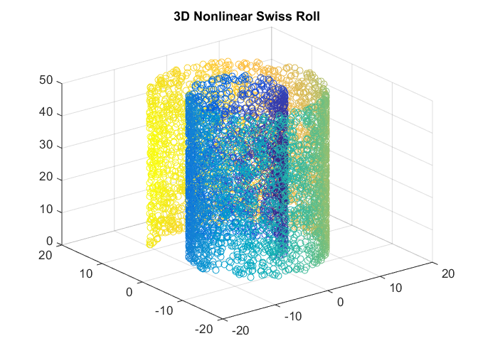
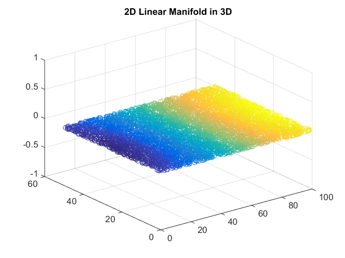
To start, take the 3D Swiss roll and its corresponding 2D points for matching.

clear;
load SwissRoll.mat
X_data=X_data(:,1:5000); %The 3D Swiss Roll
Y_data=Y_data(:,1:5000); %The 2D Plane (Generating data of Swiss Roll)
Y_data=[Y_data' zeros(1, 5000)']'; %Make the ambient dimension of the 2D plane to 3D

Check the input data by scatter plots for validation.

figure
scatter3(X_data(1,:),X_data(2,:),X_data(3,:),30,color(1:5000),'o');
title('3D Nonlinear Swiss Roll')
figure
scatter3(Y_data(1,:),Y_data(2,:),Y_data(3,:),30,color(1:5000),'o');
title('2D Linear Manifold in 3D')

Manifold Matching without Nonlinear Algorithm

Set up the parameters: tran=1000 is the number the training pairs, numData is the number of datasets to match, dimension=2 is the matching dimension, 2*tesn is the number of testing/oos points, K is the number of neighbodhood, iter=-1 uses classical MDS whenever MDS is involved.

tran=1000;numData=2;dim=2;tesn=100;K=10;iter=-1;
cc=color(1:tran+3*tesn); %Take the color scheme of Swiss roll for involved data

Formulate the data for proper input. The first 1000 data are matched training pairs, the next tesn=100 pairs are matched testing pairs, and the last tesn=100 pairs are un-matched testing pairs.

disEuc=[X_data(:,1:tran+2*tesn) [Y_data(:,1:tran+tesn) Y_data(:,tran+2*tesn+1:tran+3*tesn)]];
dis=squareform(pdist(disEuc')); %Form the distance matrix
ss=size(dis,2)/2;
dis=[dis(1:ss, 1:ss) dis(ss+1:end, ss+1:end)]; %Flatten the distance matrix for our manifold matching algorithm

First, we do Procrustes matching directly without nonlinear embedding. Note that 2*tesn points are used for testing and embedded by out-of-sample technique.

options = struct('nonlinear',0,'match',1,'neighborSize',K,'jointSelection',0,'numData',numData,'oos',2*tesn,'maxIter',iter);
[sol, dCorr]=ManifoldMatching(dis,dim,options);

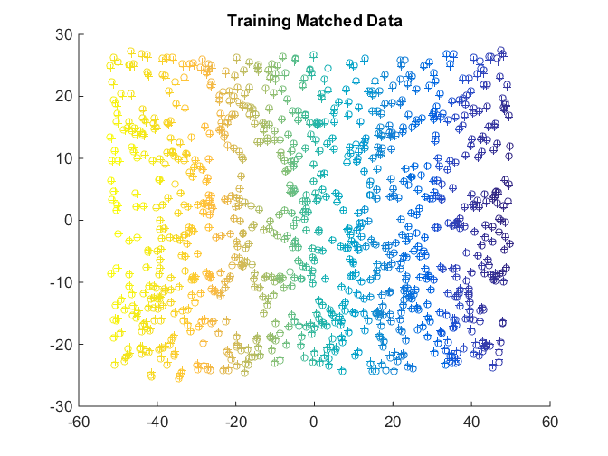
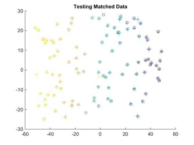
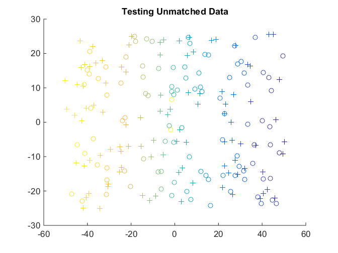
After matching, we check training data, testing matched data, and testing unmatched data using scatter plots.

figure
hold on
scatter(sol(1,1:tran),sol(2,1:tran),20,cc(1:tran),'o'); %training matched
scatter(sol(1,tran+2*tesn+1:2*tran+2*tesn),sol(2,tran+2*tesn+1:2*tran+2*tesn),20,cc(1:tran),'+');
title('Training Matched Data');
xlim([-60 60]);
ylim([-30 30]);
hold off
figure
hold on
scatter(sol(1,tran+1:tran+tesn),sol(2,tran+1:tran+tesn),30,cc(tran+1:tran+tesn),'o'); %testing matched
scatter(sol(1,2*tran+2*tesn+1:2*tran+3*tesn),sol(2,2*tran+2*tesn+1:2*tran+3*tesn),30,cc(tran+1:tran+tesn),'+');
title('Testing Matched Data');
xlim([-60 60]);
ylim([-30 30]);
hold off
figure
hold on
scatter(sol(1,tran+tesn+1:tran+2*tesn),sol(2,tran+tesn+1:tran+2*tesn),30,cc(tran+tesn+1:tran+2*tesn),'o'); %testing unmatched
scatter(sol(1,2*tran+3*tesn+1:2*tran+4*tesn),sol(2,2*tran+3*tesn+1:2*tran+4*tesn),30,cc(tran+2*tesn+1:tran+3*tesn),'+');
title('Testing Unmatched Data');
xlim([-60 60]);
ylim([-30 30]);
hold off

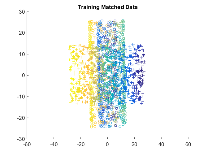
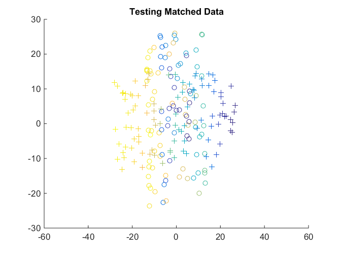
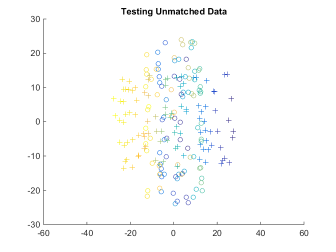
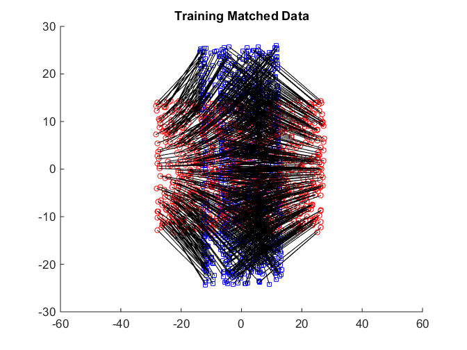
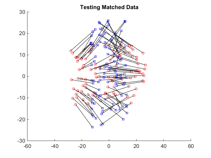
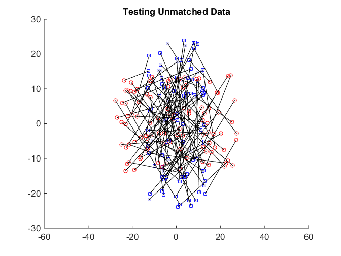
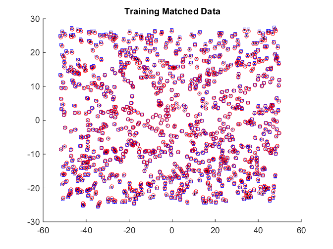
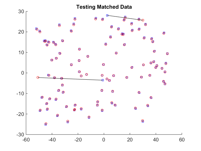
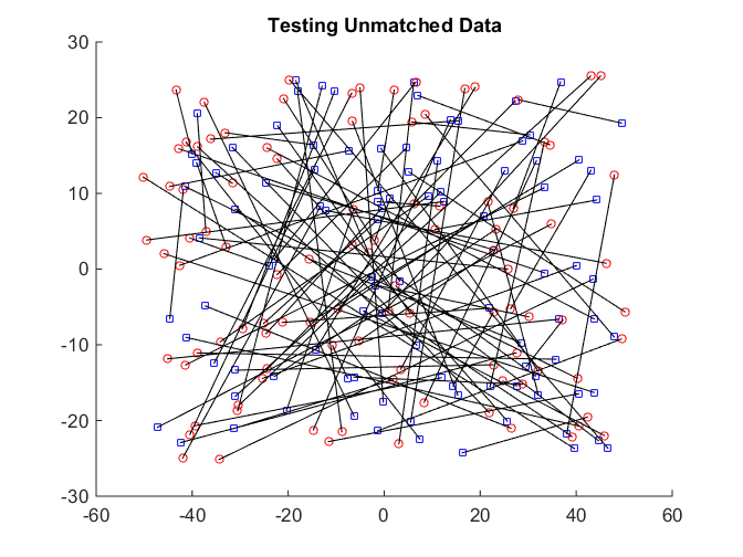
And if we check the matchedness by connecting each pair by black line, it is a mess and the matched data are never matched.

plotVelocity([sol(:,1:tran) sol(:,tran+2*tesn+1:2*tran+2*tesn)],options.numData);
title('Training Matched Data');
xlim([-60 60]);
ylim([-30 30]);
plotVelocity([sol(:,tran+1:tran+tesn) sol(:,2*tran+2*tesn+1:2*tran+3*tesn)],options.numData);
title('Testing Matched Data');
xlim([-60 60]);
ylim([-30 30]);
plotVelocity([sol(:,tran+tesn+1:tran+2*tesn) sol(:,2*tran+3*tesn+1:2*tran+4*tesn)],options.numData);
title('Testing Unmatched Data');
xlim([-60 60]);
ylim([-30 30]);

We can check the distance correlation of the training data, as well as the matching test power of the testing data at critical level 0.05. Both metrics are not too high.

dCorr
p=plotPower(sol,numData,tesn,20);
p(2)

dCorr =

    0.6404


ans =

    0.4900

Manifold Matching using Joint Isomap

Then we repeat the same procedure using joint Isomap with Procrustes matching.

options = struct('nonlinear',1,'match',1,'neighborSize',K,'jointSelection',1,'numData',numData,'oos',2*tesn,'maxIter',iter);
[sol, dCorr]=ManifoldMatching(dis,dim,options);

After matching, we again check training data, testing matched data, and testing unmatched data using scatter plots; they look much better in terms of matching, and also indicate that our embedding & oos codes should be correct in recovering the geometry.

figure
hold on
scatter(sol(1,1:tran),sol(2,1:tran),20,cc(1:tran),'o'); %training matched
scatter(sol(1,tran+2*tesn+1:2*tran+2*tesn),sol(2,tran+2*tesn+1:2*tran+2*tesn),20,cc(1:tran),'+');
title('Training Matched Data');
xlim([-60 60]);
ylim([-30 30]);
hold off
figure
hold on
scatter(sol(1,tran+1:tran+tesn),sol(2,tran+1:tran+tesn),30,cc(tran+1:tran+tesn),'o'); %testing matched
scatter(sol(1,2*tran+2*tesn+1:2*tran+3*tesn),sol(2,2*tran+2*tesn+1:2*tran+3*tesn),30,cc(tran+1:tran+tesn),'+');
title('Testing Matched Data');
xlim([-60 60]);
ylim([-30 30]);
hold off
figure
hold on
scatter(sol(1,tran+tesn+1:tran+2*tesn),sol(2,tran+tesn+1:tran+2*tesn),30,cc(tran+tesn+1:tran+2*tesn),'o'); %testing unmatched
scatter(sol(1,2*tran+3*tesn+1:2*tran+4*tesn),sol(2,2*tran+3*tesn+1:2*tran+4*tesn),30,cc(tran+2*tesn+1:tran+3*tesn),'+');
title('Testing Unmatched Data');
xlim([-60 60]);
ylim([-30 30]);
hold off

And if we check the matchedness by connecting each pair by black line, it is almost perfect (except two pairs), i.e., matched data are matched in both training and testing, and testing unmatched data are far away.

plotVelocity([sol(:,1:tran) sol(:,tran+2*tesn+1:2*tran+2*tesn)],options.numData);
title('Training Matched Data');
plotVelocity([sol(:,tran+1:tran+tesn) sol(:,2*tran+2*tesn+1:2*tran+3*tesn)],options.numData);
title('Testing Matched Data');
plotVelocity([sol(:,tran+tesn+1:tran+2*tesn) sol(:,2*tran+3*tesn+1:2*tran+4*tesn)],options.numData);
title('Testing Unmatched Data');

The distance correlation and the testing power at 0.05 are perfect.

dCorr
p=plotPower(sol,numData,tesn,20);
p(2)

dCorr =

    1.0000


ans =

     1

Manifold Matching using Separate LLE

Next we repeat the same procedure using separate LLE with Procrustes matching.

options = struct('nonlinear',2,'match',1,'neighborSize',K,'jointSelection',0,'numData',numData,'oos',2*tesn,'maxIter',iter);
[sol, dCorr]=ManifoldMatching(dis,dim,options);

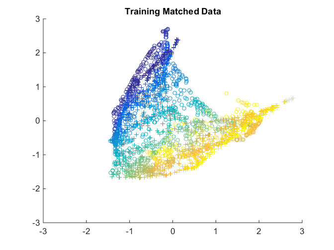
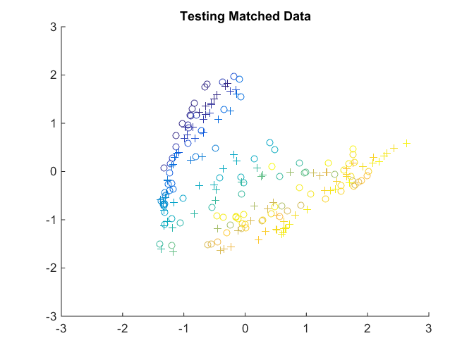
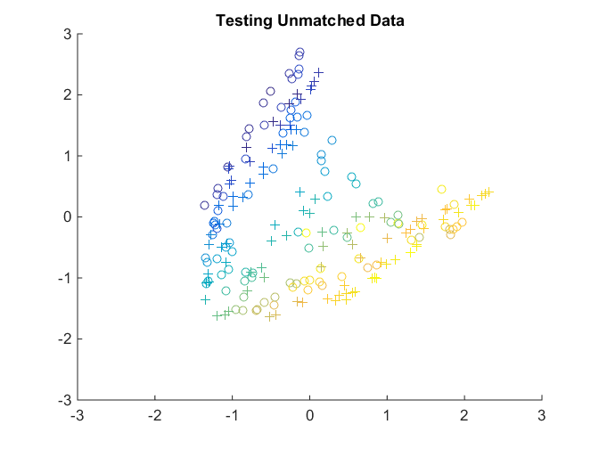
After matching, we check training data, testing matched data, and testing unmatched data using scatter plots as usual.

figure
hold on
scatter(sol(1,1:tran),sol(2,1:tran),20,cc(1:tran),'o'); %training matched
scatter(sol(1,tran+2*tesn+1:2*tran+2*tesn),sol(2,tran+2*tesn+1:2*tran+2*tesn),20,cc(1:tran),'+');
title('Training Matched Data');
xlim([-3 3]);
ylim([-3 3]);
hold off
figure
hold on
scatter(sol(1,tran+1:tran+tesn),sol(2,tran+1:tran+tesn),30,cc(tran+1:tran+tesn),'o'); %testing matched
scatter(sol(1,2*tran+2*tesn+1:2*tran+3*tesn),sol(2,2*tran+2*tesn+1:2*tran+3*tesn),30,cc(tran+1:tran+tesn),'+');
title('Testing Matched Data');
xlim([-3 3]);
ylim([-3 3]);
hold off
figure
hold on
scatter(sol(1,tran+tesn+1:tran+2*tesn),sol(2,tran+tesn+1:tran+2*tesn),30,cc(tran+tesn+1:tran+2*tesn),'o'); %testing unmatched
scatter(sol(1,2*tran+3*tesn+1:2*tran+4*tesn),sol(2,2*tran+3*tesn+1:2*tran+4*tesn),30,cc(tran+2*tesn+1:tran+3*tesn),'+');
title('Testing Unmatched Data');
xlim([-3 3]);
ylim([-3 3]);
hold off

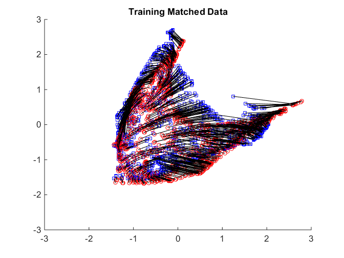
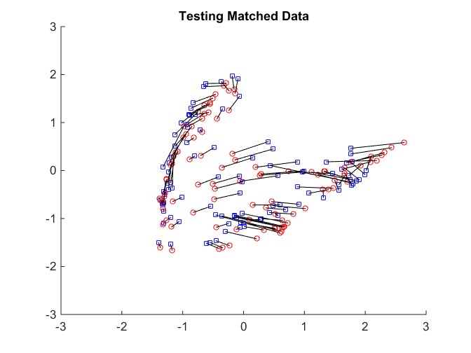
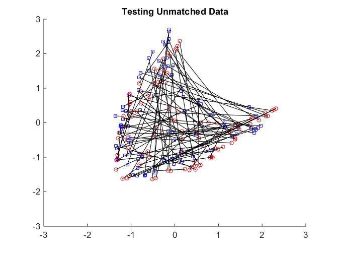
And if we check the matchedness by connecting each pair by black line, it is better than no nonlinear algorithm, but not exactly matched and worse than joint isomap.

plotVelocity([sol(:,1:tran) sol(:,tran+2*tesn+1:2*tran+2*tesn)],options.numData);
title('Training Matched Data');
xlim([-3 3]);
ylim([-3 3]);
plotVelocity([sol(:,tran+1:tran+tesn) sol(:,2*tran+2*tesn+1:2*tran+3*tesn)],options.numData);
title('Testing Matched Data');
xlim([-3 3]);
ylim([-3 3]);
plotVelocity([sol(:,tran+tesn+1:tran+2*tesn) sol(:,2*tran+3*tesn+1:2*tran+4*tesn)],options.numData);
title('Testing Unmatched Data');
xlim([-3 3]);
ylim([-3 3]);

The distance correlation and the testing power are worse than joint Isomap but better than without nonlinear algorithm. Note that if we change the jointSelection option to 1 for LLE, it will exhibit perfect matching as joint Isomap.

dCorr
p=plotPower(sol,numData,tesn,20);
p(2)

dCorr =

    0.9433


ans =

    0.8600

Manifold Matching using Laplacian Eigenmaps

At last we show how to use Laplacian eigenmaps to do matching. Note that we use the code from Laurens van der Maaten (http://lvdmaaten.github.io/drtoolbox/), and delete their outlier detection step for our matching purpose. Also OOS is not used here and all testing points are in-sample embedded, please check our paper for reasons. But if the oos option is changed to 2*tesn, the functionality is still supported, and the power will be a little lower; similarly, we can change the oos option previously to 0 for in-sample embedding.

disEuc=[X_data(:,1:tran+2*tesn) [Y_data(:,1:tran+tesn) Y_data(:,tran+2*tesn+1:tran+3*tesn)]];%nonlinear vs linear
options = struct('nonlinear',4,'match',1,'neighborSize',K,'jointSelection',0,'weight',1,'scaling',0,'numData',numData,'oos',0,'maxIter',iter);
sol=ManifoldMatchingEuc(disEuc,dim,options);

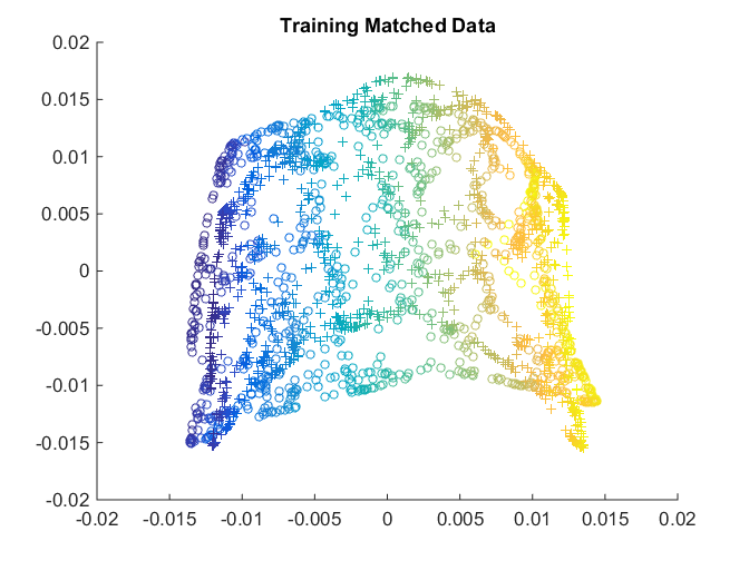
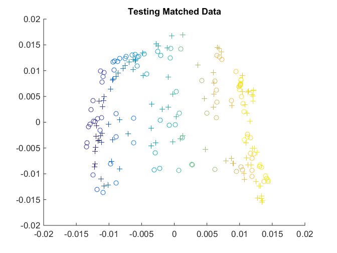
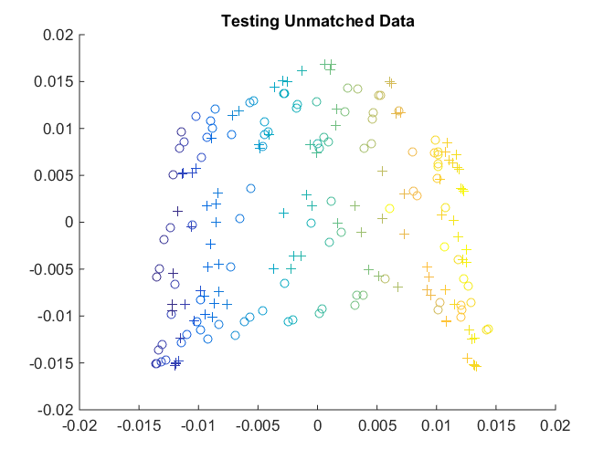
After matching, as usual, we check training data, testing matched data, and testing unmatched data using scatter plots.

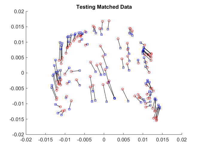
figure
hold on
scatter(sol(1,1:tran),sol(2,1:tran),20,cc(1:tran),'o'); %training matched
scatter(sol(1,tran+2*tesn+1:2*tran+2*tesn),sol(2,tran+2*tesn+1:2*tran+2*tesn),20,cc(1:tran),'+');
title('Training Matched Data');
xlim([-0.02 0.02]);
ylim([-0.02 0.02]);
hold off
figure
hold on
scatter(sol(1,tran+1:tran+tesn),sol(2,tran+1:tran+tesn),30,cc(tran+1:tran+tesn),'o'); %testing matched
scatter(sol(1,2*tran+2*tesn+1:2*tran+3*tesn),sol(2,2*tran+2*tesn+1:2*tran+3*tesn),30,cc(tran+1:tran+tesn),'+');
title('Testing Matched Data');
xlim([-0.02 0.02]);
ylim([-0.02 0.02]);
hold off
figure
hold on
scatter(sol(1,tran+tesn+1:tran+2*tesn),sol(2,tran+tesn+1:tran+2*tesn),30,cc(tran+tesn+1:tran+2*tesn),'o'); %testing unmatched
scatter(sol(1,2*tran+3*tesn+1:2*tran+4*tesn),sol(2,2*tran+3*tesn+1:2*tran+4*tesn),30,cc(tran+2*tesn+1:tran+3*tesn),'+');
title('Testing Unmatched Data');
xlim([-0.02 0.02]);
ylim([-0.02 0.02]);
hold off

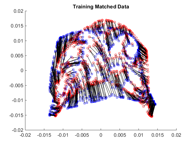
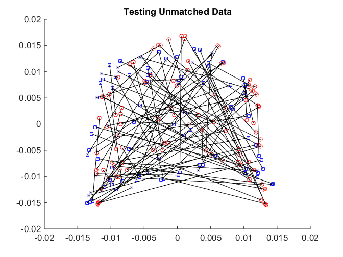
And if we check the matchedness by connecting each pair by black line, it is better than no nonlinear algorithm, but worse than joint isomap.

plotVelocity([sol(:,1:tran) sol(:,tran+2*tesn+1:2*tran+2*tesn)],options.numData);
title('Training Matched Data');
xlim([-0.02 0.02]);
ylim([-0.02 0.02]);
plotVelocity([sol(:,tran+1:tran+tesn) sol(:,2*tran+2*tesn+1:2*tran+3*tesn)],options.numData);
title('Testing Matched Data');
xlim([-0.02 0.02]);
ylim([-0.02 0.02]);
plotVelocity([sol(:,tran+tesn+1:tran+2*tesn) sol(:,2*tran+3*tesn+1:2*tran+4*tesn)],options.numData);
title('Testing Unmatched Data');
xlim([-0.02 0.02]);
ylim([-0.02 0.02]);

Our funtion does not return the distance correlation in this case, and we simply show the testing power. It is better than LLE but not perfect.

p=plotPower(sol,numData,tesn,20);
p(2)

ans =

    0.9400