The Wikipedia Matching Example

Load the Wikipedia documents English/French Text/Graph features, do manifold matching, plot the matched embedding, and calculate the distance correlation & testing power by various nonlinear embedding algorithms.

Contents

Original Dissimilarities

To start, take the dissimilarity matrices from English/French Text/Graph features for late matching. In total we have 4 data sources, named as TE, TF, GE, GF.

clear;
load ('Wiki_Data.mat','TE','TF','GE','GF');

Manifold Matching for (TE, TF) without Nonlinear Algorithm

Set up the parameters: tran=500 is the number the training pairs, numData is the number of datasets to match, dimension=10 is the matching dimension, 2*tesn is the number of testing/oos points, K is the number of neighbodhood, iter=-1 uses classical MDS whenever MDS is involved.

tran=500;numData=2;dim=10;tesn=100;K=20;iter=-1;
options = struct('numData',numData,'permutation',-1,'scaling',1);

The first 500 data are matched training pairs, the next tesn=100 pairs are matched testing pairs, and the last tesn=100 pairs are un-matched testing pairs.

[dis,~,~]=GetRealData([TE TF],0,tran,tesn,options); %This function re-organizes data for training and testing purpose

First, we do joint MDS matching directly without nonlinear embedding. Note that 2*tesn points are used for testing and embedded by out-of-sample technique.

options = struct('nonlinear',0,'match',0,'neighborSize',K,'jointSelection',0,'numData',numData,'oos',2*tesn,'maxIter',iter);
[sol, dCorr]=ManifoldMatching(dis,dim,options);

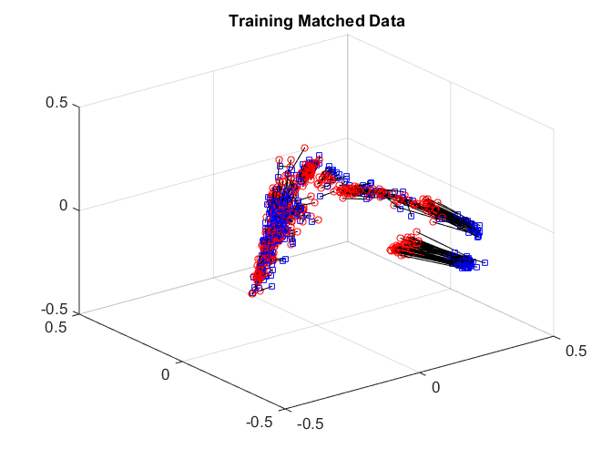
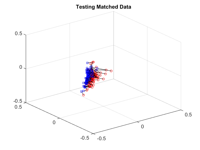
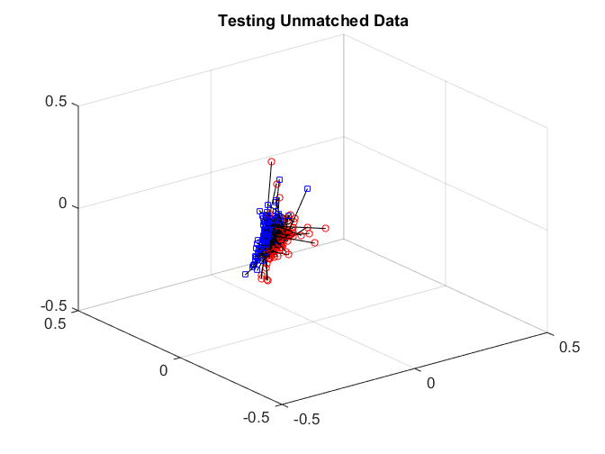
After matching, we check the matchedness by connecting each pair by black line, there are some matched patterns in the embedding. But the unmatched pairs are also well matched, dragging down the testing power.

plotVelocity([sol(:,1:tran) sol(:,tran+2*tesn+1:2*tran+2*tesn)],options.numData);
title('Training Matched Data');
xlim([-0.5 0.5])
ylim([-0.5 0.5])
zlim([-0.5 0.5])
plotVelocity([sol(:,tran+1:tran+tesn) sol(:,2*tran+2*tesn+1:2*tran+3*tesn)],options.numData);
title('Testing Matched Data');
xlim([-0.5 0.5])
ylim([-0.5 0.5])
zlim([-0.5 0.5])
plotVelocity([sol(:,tran+tesn+1:tran+2*tesn) sol(:,2*tran+3*tesn+1:2*tran+4*tesn)],options.numData);
title('Testing Unmatched Data');
xlim([-0.5 0.5])
ylim([-0.5 0.5])
zlim([-0.5 0.5])

We can check the distance correlation of the training data, as well as the matching test power of the testing data at critical level 0.05. Straight matching has a good correlation, but the testing power is not good enough.

dCorr
p=plotPower(sol,numData,tesn,20);
p(2)

dCorr =

    0.9226


ans =

    0.4700

Manifold Matching for (TE, TF) using Joint Isomap

Then we repeat the same procedure using joint Isomap with joint MDS matching.

options = struct('nonlinear',1,'match',0,'neighborSize',K,'jointSelection',1,'numData',numData,'oos',2*tesn,'maxIter',iter);
[sol, dCorr]=ManifoldMatching(dis,dim,options);

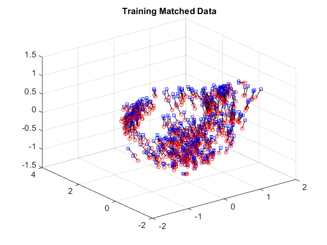
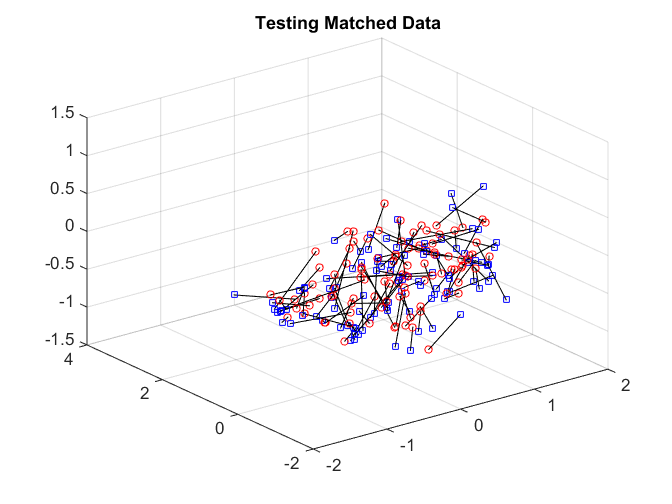
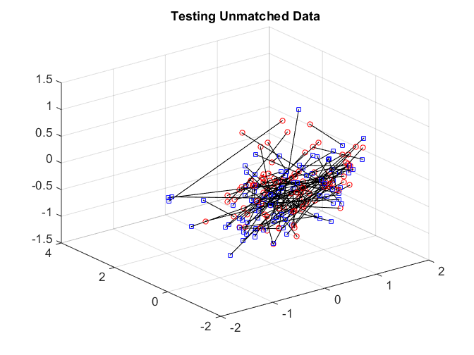
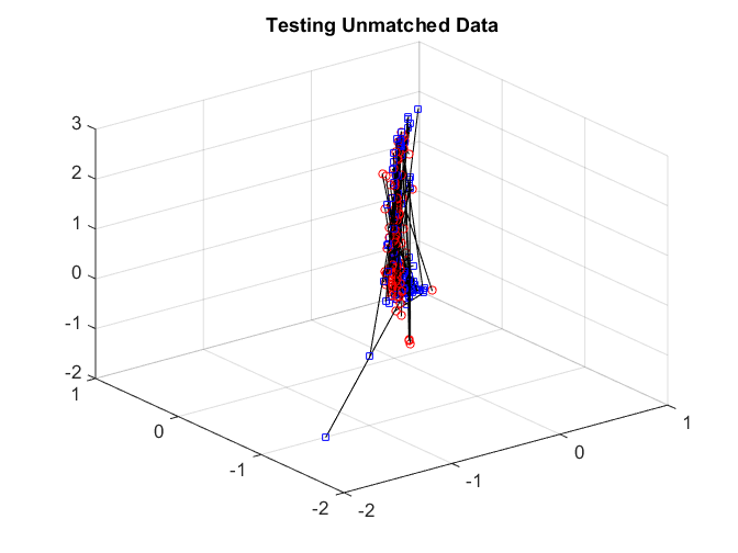
After matching, we check the matchedness by connecting each pair by black line. The training data is very well matched. The testing matched pairs are reasonably matched with the testing unmatched pairs being clearly unmatched. This improves the testing power.

plotVelocity([sol(:,1:tran) sol(:,tran+2*tesn+1:2*tran+2*tesn)],options.numData);
title('Training Matched Data');
xlim([-2 2])
ylim([-2 4])
zlim([-1.5 1.5])
plotVelocity([sol(:,tran+1:tran+tesn) sol(:,2*tran+2*tesn+1:2*tran+3*tesn)],options.numData);
title('Testing Matched Data');
xlim([-2 2])
ylim([-2 4])
zlim([-1.5 1.5])
plotVelocity([sol(:,tran+tesn+1:tran+2*tesn) sol(:,2*tran+3*tesn+1:2*tran+4*tesn)],options.numData);
title('Testing Unmatched Data');
xlim([-2 2])
ylim([-2 4])
zlim([-1.5 1.5])

The distance correlation and the testing power are both better comparing to no nonlinear algorithm.

dCorr
p=plotPower(sol,numData,tesn,20);
p(2)

dCorr =

    0.9843


ans =

    0.7800

Manifold Matching for (TE, TF) using Separate LLE

Next we repeat the same procedure using separate LLE with Joint MDS matching.

options = struct('nonlinear',2,'match',0,'neighborSize',K,'jointSelection',0,'numData',numData,'oos',2*tesn,'maxIter',iter);
[sol, dCorr]=ManifoldMatching(dis,dim,options);

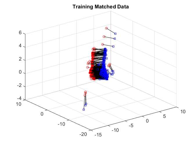
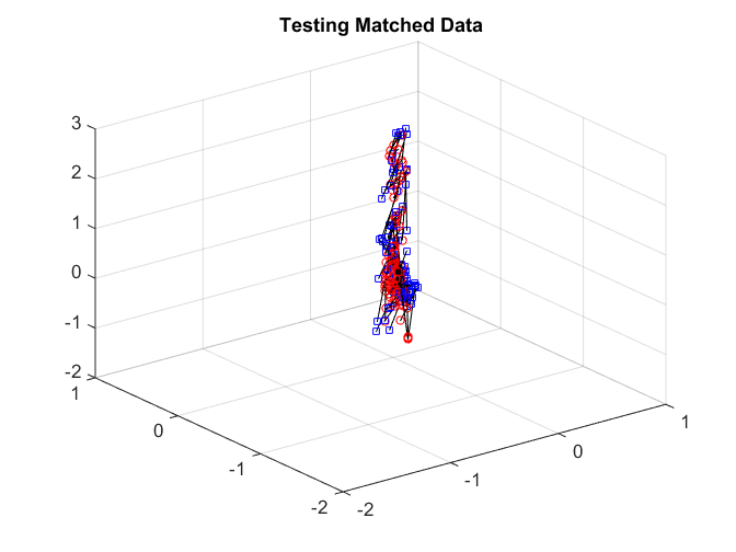
After matching, we again check the matchedness by connecting each pair by black line. The testing data are quite difficult to distinguish.

plotVelocity([sol(:,1:tran) sol(:,tran+2*tesn+1:2*tran+2*tesn)],options.numData);
title('Training Matched Data');
plotVelocity([sol(:,tran+1:tran+tesn) sol(:,2*tran+2*tesn+1:2*tran+3*tesn)],options.numData);
title('Testing Matched Data');
xlim([-2 1])
ylim([-2 1])
zlim([-2 3])
plotVelocity([sol(:,tran+tesn+1:tran+2*tesn) sol(:,2*tran+3*tesn+1:2*tran+4*tesn)],options.numData);
title('Testing Unmatched Data');
xlim([-2 1])
ylim([-2 1])
zlim([-2 3])

Both the distance correlation on the training data and the matching test power are significantly worse than joint Isomap.

dCorr
p=plotPower(sol,numData,tesn,20);
p(2)

dCorr =

    0.8584


ans =

    0.5000

Manifold Matching for (TE, TF, GE) without Nonlinear Algorithm

At last, we show a three dataset matching example, using almost the same parameters except changing numData to 3.

tran=500;numData=3;dim=10;tesn=100;K=20;iter=-1;
options = struct('numData',numData,'permutation',-1,'scaling',1);
[dis,~,~]=GetRealData([TE TF GE],0,tran,tesn,options); %This function re-organizes data for training and testing purpose

We do joint MDS matching directly without nonlinear embedding, and just check the distance correlation and testing power.

options = struct('nonlinear',0,'match',0,'neighborSize',K,'jointSelection',0,'numData',numData,'oos',2*tesn,'maxIter',iter);
[sol, dCorr]=ManifoldMatching(dis,dim,options);
dCorr
p=plotPower(sol,numData,tesn,20);
p(2)

dCorr =

    2.1105


ans =

    0.4400

Manifold Matching for (TE, TF, GE) using Joint Isomap

Then we repeat the same procedure using joint Isomap with joint MDS matching, and check the distance correlation and testing power. They are much better using joint isomap than no nonlinear algorithm.

options = struct('nonlinear',1,'match',0,'neighborSize',K,'jointSelection',1,'numData',numData,'oos',2*tesn,'maxIter',iter);
[sol, dCorr]=ManifoldMatching(dis,dim,options);
dCorr
p=plotPower(sol,numData,tesn,20);
p(2)

dCorr =

    2.7116


ans =

    0.9200

All the above experiments can be repeated; which we repeat 100 times in our paper for randomly selected data for testing.

Published with MATLAB® R2014b